Chapter 2: Casing Design lec ( 6 )


Open Hole Completions

The first decision on casing the pay zone is not of size or weight but whether or not to run casing at all. Open hole completions represent the simplest type of completions and have some very useful traits. They also present some problems. An open hole or barefoot completion is usually made by drilling to the top of the pay, then running and cementing casing. After these operations, the pay is drilled with a nondamaging fluid. Since the other formations are behind pipe, the drilling fluid overbalance is only that needed to control the reservoir pressure. This creates less damage. Open hole completions have the largest possible formation contact with the wellbore, allowing injection or production with every part of the contacted interval. The effect of the open hole on stimulated operations depends on the type of job. Fracturing operations are often easier in the open hole than through perforations by less possibility of perforation screenouts, but the perforations may make the zone easier to break down since a crack (the perforation) has already been placed. Matrix acidizing can more evenly contact the entire zone in an open hole but is more difficult to direct by straddle packer than in a cased hole. Hydraulic jetting is most effective in the open hole. Productivity of open hole gravel packs, especially the underreamed open holes are usually much higher than cased hole gravel packs. Why then, are casing strings even used? Part of the answer is in formation (wellbore) stability concerns and part is unfamiliarity with completing and producing the open hole completions. A decision must be reached on the merits of the completions on the pay in question. If the pay is prone to brittle
failures during production that leads to fill, most operators choose to case and cement. In areas of water coning or zone conformance problems, casing may make isolation of middle or top zones possible. With the advent of improved inflatable packers and matrix sealants, however, isolation is also possible in open holes, although wellbore diameter may be severely restricted.

Cased Hole Completions

A casing string is run to prevent the collapse of the wellbore and to act in concert with the cement sheath to isolate and separate the productive formations. The size of the casing is optimized on the expected productivity of the well and must be designed to withstand the internal and external pressures associated with completion, any corrosive influences, and the forces associated with running the casing.
An optimum design for a casing string is one designed from "the inside out", a design that is based on supplying a stable casing string of a size to optimize total fluid production over the life of the well (including possibility of secondary or tertiary floods). The effective design of a casing string for any well consists of four principal steps.

1. Determine the length and size of all casing strings that are needed to produce the well to its maximum potential.
2. Calculate the pressure and loads from predicted production and operations such as stimulation, thermal application and secondary recovery.
3. Determine any corrosive atmosphere that the casing string will be subjected to and either select alloys which can resist corrosion or design an alternate corrosion control system.
4. Determine the weight and grade of casing that will satisfactorily resist all of the mechanical, hydraulic, and chemical forces applied.

The sizing of a casing string must be complete before finalizing the bit program during the planning of the well. A casing string can be visualized as a very long telescoping tube with the surface casing or conductor pipe as the first segment and the deepest production string or liner as the smallest, most extended section. Each successive (deeper) segment of the casing string must pass through the last section with enough clearance to avoid sticking. Figure 2.1 illustrates the way the casing string fits together. The drill bits used for each section are usually 1.5 to 3 in. or more larger than the casing 0.d. to be run. When one section is cased and cemented, a bit just small enough to pass through the casing
drift ID is run to drill to the next casing seat (casing shoe set depth). During drilling, departing from the bit program is often required, especially in a wildcat when the fluid pressures in the formations cannot be controlled with a single mud weight without either breaking down some formations by hydraulic fracturing with the mud, or allowing input of fluid from other formations because of low hydrostatic drilling mud pressure (a kick). Ideally, just before this noncontrollable point is reached, the “casing point” is designated and a casing string is run. Economics of drilling and cementing dictate that these casing points be as far apart as formation pressures and hole stability will allow. Use of as few casing strings as possible also permits larger casing to be used across the production zone without
using extremely large diameter surface strings.


Use of small casing severely restricts the opportunities for deepening the well or using larger pumps. Use of small casing to save on drilling costs is usually a poor choice in any area in which high production rates (including water floods) are expected.

Description of Casing Strings

There are several different casing strings that are run during the completion of a well. These strings vary in design, material of construction and purpose. The following paragraphs are brief descriptions of the common required strings and specialty equipment.
 The conductor pipe is the first casing which is run in the well. This casing is usually large diameter and may be set with the ”spudding” arm on the rig (The spudding arm drives in the casing.). The primary purpose of the conductor casing is as a flow line to allow mud to return to the pits and to stabilize the upper part of a hole that may be composed of loose soil. The depth of the conductor pipe is usually in the range of 50-250 ft with the depth set by surface rocks and soil behavior. It also provides a point for the installation of a blow-out preventer (BOP) or other type of diverter system. This allows any shallow
fluid flows to be diverted away from the rig, and is a necessary safety factor in almost all areas. In areas with very soft and unconsolidated sediments, a temporary outer string, called a stove pipe, may be driven into place to hold the sediment near the surface.
The well is drilled out from the conductor pipe to a depth below the shallow fresh water sands. The surface casing string is run through the conductor pipe and has three basic functions: (1) it protects shallow, fresh-water sands from contamination by drilling fluids, (2) prevents mud from being cut with brines or other water that may flow into the wellbore during drilling, and (3) it provides sufficient protection of the zone to avoid fracturing of the upper hole so that the drilling may proceed to the next casing point. This surface casing is cemented in place over the full length of the string and is the second line of safety for sealing the well and handling any high pressure flow. The intermediate string is the next string of casing, and it is usually in place and cemented before the higher mud weights are used. It allows control of the well if subsurface pressure higher than the mud
weight occurs and inflow of fluids is encountered. This inflow of well fluids during drilling or completion of the well is called a kick and may be extremely hazardous if the flowing fluids are flammable or contain hydrogen sulfide (sour gas). The intermediate casing may or may not be cemented in place and, if not cemented, may be removed from the well if an open-hole completion is desired. If a casing string is not hung from the surface, but rather hung from some point down hole, it is called a “liner”. In most wells, the top of the liner is cemented in place to provide sealing. The top of the liner is set inside an upper casing string. The section where the liner runs inside another string is the overlap
section. Production liners are permanent liners that are run through the productive interval. On some occasions] they may be run back to surface in a liner tieback operation. The tieback consists of a downhole mechanical sealing assembly in a hanger into which a linear string or the tie back string is “stabbed” to complete the seal. A cement job seals the liner into place in the casing and prevents leakage from the formation into the casing. The lower part of the casing string, into which the liner is cemented, is called the overlap section. Overlap length is usually only enough to insure a good seal, typically 300 to
500 ft. Overlap length may be longer where water or gas channeling would create a severe problem. Liners are run for a variety of reasons. If the operator wants to test a lower zone of dubious commercial quality, a liner can be set at less expense than a full casing string. Also, in lower pressure areas where multiple strings of pipe up to the surface are not necessary to control corrosion or pressure, the liner can be an expense-saving item. In wells that are to be pumped by ESP’s (Electric Submersible Pumps), the liner through the production section leaves full hole diameter in the casing string above the pay for setting large pumps and equipment. The production casing, or the final casing run into the well, is a string across the producing zone that is hung from the surface and may be completely cemented to the surface. This string must be able to withstand the full wellhead shutin pressure if the tubing or the packer fails. Also, it must contain the full bottomhole pressure and any mud or workover fluid kill weight when the tubing or packer is removed or replaced during workovers. The decision on whether to cement the full string is based on pressure
control, economics, corrosion problems, pollution possibilities and government regulations.

Casing Clearance

The necessary clearance between the outside of the casing and the drilled hole will depend on the hole and mud condition. In cases where mud conditioning is good or the mud is lightweight and the formations are competent, a clearance of 1.5 in. total diameter difference is acceptable. For this clearance to be usable, the casing string should be short. Primary cementing operations may not be successful in this clearance and cementing backpressures will be high. A better clearance for general purpose well completions is 2 to 3 in. For higher mud weights, poorer mud conditioning, poor quality hole and higher formation pressures, clearance should be increased. For more information on hole quality and sticking, review the chapter on Drilling the Pay. Excessive clearances should also be
avoided. If the annular area is too large, the cement cannot effectively displace the drilling mud.
A reference for hole size and casing size for single or multiple string operations are shown in
Figure 2.2.2 The solid lines indicate the common biffcasing combinations with adequate clearance for most operations. The dashed lines indicate less common (tighter) hole sizes or bitkasing combinations. Long runs of casing through close clearance holes usually leads to problems. Tight clearances should be avoided where possible.


Connections
The threaded connection of casing or tubing is important because of strength and sealing considerations. The connections are isolated pressure vessels that contain threads, seals and stop shoulder^.^ The fluid seal produced by a connection may be created in the threads by a pipe dope fluid or by a metal or elastomer seal within the connection. Strength of the connection may range from less than pipe body strength to tensile effciencies of over 11 5% of pipe body ~t rengthT.~hr eads are tapered and designed to fit a matching thread in a particular collar. In the API round thread series, the connection may be either short thread and coupling (ST&C) or long thread and coupling (LT&C) as illustrated in Figure 2.3. If the thread is an eight round, it means eight threads per inch. The length description
refers to the relative length of the coupling and the amount of pipe that is threaded (the pin). Creation of a pressure tight seal with an API round thread requires filling the voids between the threads with a sealing compound (thread dope) during makeup of the joint.


Although the standard 8-round threaded connection is reasonably strong, it does not approach the strength of the body of the pipe. As tensile loads increase toward the limit of the pipe, the connection will normally fail by shearing off the threads from the pipe or by thread jumpout caused by pipe deformation under severe loads.
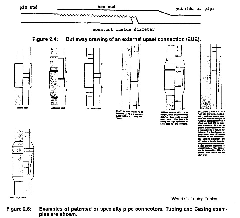
To make a stronger joint in tubing, a thicker (larger outside diameter) section is left at the end of the pipe so that threads can be cut without making the wall thickness of the pipe thinner than in the body. This form of connection is called external upset or EUE, Figure 2.4. Its inside diameter is the same as the pipe. A nonupset, or NU pipe and several other joint types are shown in Figure 2.5 The outside diameter of the EUE joint is larger than the NU connection, and the coupling or collar is normally manufactured on the pipe. Another method of increasing the strength of the threaded connection is by upsetting the connection to the inside of the pipe. This internal upset restricts the inside diameter of the pipe at every joint and is only used in drill pipe where a constant outside diameter is necessary.
Other sealing surfaces are available in special connections and have found popularity where rapidly made, leak free sealing is important. The two-step thread connection uses two sets of threads with a metal sealing surface between. In other connections, a groove at the base of the box may contain an elastomer seal. A variety of connection types and sealing surfaces are available, Figure 2.5. The disadvantage to the numerous thread and sealing combinations is that the connections cannot be mixed


in a string without crossovers (adaptors). A more detailed discussion of connections are available from other sources.

Chapter I : Drilling the Pay, Selecting the Interval and the Initial Design con't lec ( 5 )

Coiled Tubing Drilling
In addition to jointed pipe drilling, coiled tubing (see Chapter 18 for Coiled Tubing quipment and Techniques) can also be used for drilling and milling in some applications. Coiled tubing offers several advantages and a few current disadvantages that should be explored for their potential in completions and workovers. One of the best uses of coiled tubing drilling may be in combination with underbalanced drilling “where the well is allowed to flow during the drilling operation.”
The simplest coiled tubing drilling bottomhole assembly (BHA) includes a bit, mud motor, stabilizers or collars, the connector and the coil. The abilities of coiled tubing for drilling include a continuously fed fluid transfer mechanism (the coil) with no tool joints. This one feature allows the smooth external wall that can be sealed very easily at the surface. Fluids returning from downhole up the annular area are vented under pressure to surface separation equipment and small kicks and gases can be handled easily.
In many of the first examples of coiled tubing milling and drilling, the mud motors which provide turning ability at bit often stalled or stopped turning because of excess loads placed on the bits from either the string or the bottomhole assembly. This reoccurring motor stalling problem resulted in very slow penetration. Motor stalls typically occur when downward forces (weight and force) at the bit are greater than the ability of the motor to turn the bit. There are a number of reasons for motor stalls.
      1. Too aggressive a bit or mill design will require excessive power to turn. Less aggressive (smaller teeth) milled and bits are easier to turn, although they may drill some materials slightly slower.
      2. Coiled tubing milling and drilling typically uses smaller motors with less torque. The smaller motor design utilizes very small clearances and small loaders and stators in the mud motors.
      3. In deviated wells, trying to apply force on coiled tubing from the surface may result in first sinusoidal and then helical buckling. When buckling occurs, regardless of its location in the wellbore, the stored energy will try to work its way either up or down and add an extra force against the bit the surface unit.
      4. The injector feed control at the surface is often a major source of the problem. The injector is a source of all upward and downward force exclusive of drill collars and other weight. Ideally, the feed of the coiled tubing through the injector should be no faster than the penetration through the bit or mill. If too much tubing runs through the injector at any time, the total force on the bit increases and a motor stall may occur. For best results, very slow speed or micro movement of the injector head should be possible in any unit used for coiled tubing drilling.

Underbalanced Drilling

Traditionally the main goal of any drilling operation was to keep control of the well. This resulted in a positive pressure from the wellbore outward into the formation stopping the inward flow of all reservoir fluids. Underbalanced drilling with a pressure contained system allows the formation fluids to flow into the wellbore and prevents invasion of the drilling fluids into the formation. Although this method is more difficult to handle with its increasing amount of fluid recovery, it does provide the very best method of damage-free drilling. The elements of an underbalanced drilling system include a contained, safe, surface system that can separate solids, liquids and gases. This type of a separator system generally uses solid separation equipment and a horizontal separator to separate liquids and gases. Other important aspects of underbalanced drilling include adequate hydraulics of the fluid circulation system to allow bit lubrication, cooling and hole cleaning, plus sufficient pressure in the wellbore to prevent full-scale hole unloading. Typically, underbalanced drilling attempts to maintain from 112-2 Ib per gal under the pore pressure. Depending on the permeability of the formation and the type of fluids flowing, the pressure might have to be adjusted to keep the solid separation facilities within their reasonable operating limits.

Slimholes

Slimhole drilling has become a popular concept in recent years. Although smaller diameter holes are theoretically cheaper to drill because less formation is actually removed, they are not always a cheaper hole to drill. Cost of drilling involves not only the time to cut through a part of the formation, but also involves the use of existing (paid for) versus new and smaller equipment, and several other factors including pressure control and the cost of the completion. Many times it has been found that drilling a smaller hole actually costs more than drilling a traditional hole where costs of normal sized equipments was very cheap in comparison to special ordered newer and smaller equipment. Pressure control during drilling or workovers in small wellbores is often very difficult. An example, shown in Chapter 15 on workover fluids and control, shows that the volume of a 1 bbl kick in a small
diameter (3-3/4 in. hole) versus a large diameter hole (9-112 in.) may result in several hundred psi difference just from the volume of the hole filled by the 1 bbl kick. When drilling or working over holes with small diameters, accurate trip tanks and a functional alarm system must be used to minimize danger from kicks.

Initial Completion Design

Selecting the Pay Zone
Selecting the pay and deciding where to place the wellbore are two of the most important pieces of engineering that most occur in the completion process. Many rocks from shales to fractured granites contain hydrocarbons, but, not every rock type or reservoir can qualify as a pay zone. Selection of the pay breaks down into several basic considerations:

1-Prospect development economics,
2-porosity and permeability requirements,
3-hydrocarbon type and saturation requirements,
4-recoverable hydrocarbon volumes (by primary, secondary and tertiary methods),
5-pressure support,
6-reservoir stability,
7-recognition of compartmentalization,
8-availability of technology to cost effectively produce the reserves,
9-ability to plug and abandon the reservoir,
10-environmental and other risks.

The economics of a project depend simply on whether enough money can be made from sale of the productive hydrocarbons in a limited amount of time to offset the total costs of the project. The associated cost of the project may include a variety of finding, development, production and abandonment costs. Among these costs are: prospect leasing, field development, field operation, royalties, interests on the money used,
profit, risks, plug and abandonment costs and contingency funds for all matters problems such as blowouts and cleanup operations. Substantial deposits of crude oil and gas are known in many parts of the world, bu cannot be currently produced because the production rates cannot offset the cost of development and operation. Every year many of these (outer limit) deposits are being brought on-line as producing reservoirs as technology is being developed or the cost of development drops through other factors. Even the cost of
Deepwater developments, for example, which can be in the hundreds of millions or even billions of dollars can be economic if risk can be reduced and if the production rate from the wells is high. Every project from the shallowest stripper well at 2 bpd to the 100 mmscf/d or 30,000 bpd oil wells must be judged by some risks versus cost recovery and profit factor.
Porosity and permeability are the reservoir storage and pathway of flowing fluids. Porosity is the void space between the grains in which fluids can be stored. Permeability is a measurement of the ability of fluids to flow through the formation. Rocksuch as shales and chalk, for example, may have extremely high porosities approaching 30-40 percent, but the porosity is not linked together, thus the permeability is very low. On the other hand, naturally fractured formations may have extremely high permeabilities approaching tens of darcies
in some cases, but have very low porosity, often only 4-6 percent. The amount of porosity and permeability necessary for a project depends on the production rate needs, although, operations such as hydraulic fracturing can increase the production rate of a well by a factor of 2 to 10 or more. Fracturing alone may not make the project economic. The economics of a project are such that every factor must be weighed in turn in the economic justification and critical factors, such as hydrocarbon storage and the permeable pathway, must be available before even a huge reservoir with billions of barrels of oil can be made productive. In reservoir selection, often times a porosity or permeability cutoff is used for pay versus nonpay identification. Recognition of this level from porosity logs and flow tests are often critical in establishing minimum pay requirements.
Hydrocarbon type and saturation determine the amount of hydrocarbons that may occupy the pore space of a reservoir. Many factors such as moveable versus irreducible saturations and changing factors such as relative permeability can make the saturation and permeability values “moving targets.” There are no set minimum values for hydrocarbon saturation, however, the best parts of the reservoir will usually have the higher values of hydrocarbon saturation. Saturation of water may also be a key in pay identification. Extremely high saturations of water may indicate hydrocarbon depletion or movement of an aquifer into the
Pay.
The recoverable hydrocarbon volumes are usually calculated form the measured values of porosity and saturation. Oil in place quantities do not indicate that all of that oil can be recovered. The porosity of a formation varies from very large pores to very small pores and the oil in very small pores often will not flow from the small capillaries even under very high depletion pressures. How much oil will flow from a rock is dependent on the size of the pore spaces, the oil saturation and type and the amount of energy available to push the
oil towards the wellbore. Recoverable hydrocarbon estimates may vary many percentage points from what reality shows later on. The differences many times are in how well the pressure supports the drive mechanism in producing the fluids.
The pressures in the reservoir dictate how much fluid will ultimately be recovered. Many different types of pressure supports are available. The typical pressure support mechanisms include bottom and edgewater drives, gas cap drives, volumetric depletion and other pressure sources such as reservoir compaction and other factors. Each of these pressure support mechanisms has advantages and disadvantages to deciding recovery in a reservoir. Among the most effective types of reservoir pressure support are the bottom and
edgewater drives. These systems may maintain pressure at initial values clear to the end of the project. The problems with them is they may produce large amounts of water along with the oil. Volumetric depletion is usually found in a sealed reservoir and then the reservoir may deplete without producing any water. The recovery, however, from this types of reservoir is extremely low, since reservoir energy bleeds off very quickly. Pressure support can be added, in some cases, by the use of water floods, gas repressurization or
other types of pressure maintenance such as tertiary floods. When factors such as bottomwater or edgewater drive are recognized early, the location of the wellbores can be selected to take advantage of flow paths of the drive fluids and recoveries can be enhanced.
Reservoir stability is an issue which may effect the initial completion or repairs or recompletions throughout the life of the reservoir. Many geologically young formations lack sufficient strength for formation coherency during all phases of production. Recognition of this stability issue is usually easy because of rapid drilling rates, sand strength issues in the wellbore or other factors. The decision on adding a stabilizing completion
is usually made after consideration from initial flow tests and other factors. The most common methods of include resign consolidation or production rate restriction to avoid sanding. Recognition of compartmentalization is probably one of the most important factors in the initial design of well completions for a project. Compartmentalization is the division of a reservoir into partial or fully pressure isolated compartments by faults, permeability or porosity pinchouts, folding, shale streaks, barriers or other factors. When  compartmentalization is recognized, the location and type of wellbores can be selected to
efficiently drain the compartments and to take advantage of fluid flow patterns within the reservoir. Many of the failures of even large fields can be traced to a failure to recognize compartmentalization during the early development steps in the reservoir. The availability of technology to produce the reserves is an area which keeps the oil industry active in
research and development. Technology such as water flooding, hydraulic fracturing, artificial lift, cold flow of heavy oils, coal degassification and many other projects have increased the worlds recoverable hydrocarbons and continue to be a critical part of meeting the worlds energy needs. When the reservoir flow patterns and other factors are understood, technology can often be developed within a moderate time frame to meet needs in specialized reservoirs. The ability to produce hydrocarbons should never outstrip the ability to control the flow or the ability to plug an abandoned reservoir. Plug and abandonment intentions must take into account that the reservoir should be left in as good a condition as possible for potential tertiary operations that may recover even more fluids. Plug and abandonment costs can be a significant amount of the project cost. Offshore plug and abandonment of fields may reach over 100 million dollars. There are many associated risks, both political and environmental in developing and producing a hydrocarbon depositry. These risks must be taken into account during the economic justification for the reservoir and should offer as good a solution as is possible to the legitimate concerns posed in any situation. Once the values are known, selection of the pay can begin. The selection process uses a number of pieces of information gathered by electronics and other factors.
The objectives in this chapter will be to establish ground rules about what general completion mechanisms have the best fit to the reservoir potential.
Completion design is a function of reservoir characteristics. The problem is that reservoir data, particularly the design sensitive data such as permeability, porosity, saturations, pressure, barriers and longevity, are only fully available after most of the wells in the field have been drilled, completed and tested. In many cases, after initial drilling and completion, reservoir barriers are finally recognized and extreme redrilling or stimulations are needed to process the reservoir. The key to a good initial completion is to collect and assess the data at the earliest possible time, to allow the best early choice of completion.
Successful completions recognize the flow characteristics of the reservoir. There are a number of completion possibilities; each with a limited “fit” to the reservoir properties. The following is a general listing of the completion types with a few of the reservoir variables. The numbers for most variables are typical but only general estimates.

Vertical well
open hole
natural completion
High permeability (Kh 2 10 md for oil, 1 1 md for gas) stable formation (no movement or spalling) no bottom or edge water drives low KJK, c 0.5 KH) (or deviated wells not considered possible) no fracture plannedlpossible, no limits on surface reservoir access
laminations not “frequent.”


Special considerations:
1. Steeply tilting pay: examine hydrocarbon and water fluid flow path to wellbore including effects of K, and KH. Also investigate fracture growth and path. May choose uphill horizontal wellbore to go after “attic” or up-dip reserves that are above vertical well contact.
2. High permeability “streaks”: The size and permeability contrast to the reservoir location with respect to oil/water contact can significantly affect production or water break through. Orientation of the well path or decision to frac may be affected.
3. Salt or techtonic forces: Salt Ylow” may produce extreme loads on casing. The normal approach requires concentric dual casing strings with annular spaces cemented. Techtonic forces, and some horizontal collapse forces may create point loads on the casing which are better handled by extremely heavy wall casing strings.
4. Sweep/Floods: Well placement to process a reservoir uses the permeability pathways for best advantage. Wellbore location, orientation and deviation may be influenced.
5. Fluid Requirements: Heavy oil, scaling, organic precipitation, chronic emulsions, bubble and dew points and other special requirements may make completion compromises or redesigns necessary.
6. Multiple Zones: multiple zones completions and independent completions may be required by pressure, fluid or royalty owners.
7. The initial design is the starting place for the completion, however, it should never be construed to be unchangable. Flexibility is required for any completion to take advantage of information that can be obtained from drilling or other sources.

Concepts in Crop Rotations

1. Introduction
1.1 Crop rotations – A historical perspective
Crop rotation is the production of different economically important plant species in
recurrent succession on a particular field or group of fields. It is an agricultural practice that
has been followed at least since the Middle Ages. During the rule of Charlemagne crop
rotation was vital to much of Europe which at that time followed a two-field rotation of
seeding one field one year with a crop and leaving another fallow. The following year the
fields were reversed (Butt, 2002). Sometime during the Carolingian period the three-field
rotation system was introduced. It consisted of planting one field, usually with a winter
cereal, a second with a summer annual legume, and leaving a third field fallow. The
following year a switch would occur. Sometime during the 17th and /or 18th centuries it was
discovered that planting a legume in the field coming out of fallow of the three-field rotation
would increase fodder for livestock and improve land quality, which was later found to be
due to increased levels of available soil nitrogen (N). During the 16th century Charles
Townshend 2nd Viscount Townshend (aka Turnip Townshend) introduced the four-field
concept of crop rotation to the Waasland region of England (Ashton, 1948). This system,
which consisted of a root crop (turnips (Brassica rapa var. rapa)), wheat (Triticum aestivum
L.), barley (Hordeum vulgare L.), and clover (Trifolium spp.) followed by fallow. Every third
year introduced a fodder crop and grazing crop into the system, allowing livestock
production the year-round and thus increased overall agriculture production. Our present
day systems of crop rotation have their beginnings traceable to the Norfolk four-year
system, developed in Norfolk County England around 1730 (Martin, et al., 1976). This
system was similar to that developed by Townshend except barley followed turnips, clover
was seeded for the third year and finally wheat on the fourth year. The field would then be
seeded to turnips again with no fallow year being part of the rotation.
In the new world, prior to the arrival of European settlers, the indigenous people in what is
now the Northeastern United States, practiced slash-and-burn agriculture combined with
fishing, hunting, and gathering (Lyng, 2011). Fields were moved often as the soil would
become depleted and despite the tale of Native Americans teaching the European settlers to
put a fish into the corn hills at planting, there is little or no evidence of the aboriginal people
fertilizing their crops. Maize would be planted in hills using crude wooden hoes with
gourds and beans (Phaseolus spp. L.) being planting alongside and allowed to climb the
maize stalks. When an area would become depleted of plant nutrients, it would be
abandoned and over time, would recover its natural fertility. Lyng (2011), describes the
Native Americans of the northeast as not so much conscience ecologist but rather people
with a strong sense of dependences on nature minus the pressure to provide for consumer
demands. Plains Indians on the other hand are classified as being of two cultures. There
were the nomadic nations that followed the herds of bison that roamed the region and lived
mainly on a diet of bison meat and what they might gather in the way of wild berries, fruits,
and nuts with very little farming except for some maize and tobacco (Nicotiana tabacum L.).
There were then the nations that lived on a combination of meat and crops they would raise.
These peoples tended to live in established villages and would fish, hunt, and gather wild
fruit and berries. The crop farming they practiced again, were maize, beans, and squash
(Cucubina spp. L.), sometimes referred to as “The Three Sisters” in Native American society
(Vivian, 2001). As with the nations in what would become the northeastern United States,
the Plains Indians that practiced crop farming would usually clear their garden areas by
slash and burn, grow their crops, and then allow a two-year fallow before planting again.
Just prior to planting, some villages would carry in brush and other plant debris to burn
along with the refuge that grew in the field during fallow to “enrich” the soil for the crops
about to be planted.
The early European settlers attempted to raise those crops (wheat, and rye (Secale cereal L.))
which they were accustom to, using cultivation methods they had used in the old country.
They also, introduced livestock, (cattle, swine, and sheep) which were not found in the New
World but that had been a major source of food for them in their native homeland. They
soon discovered that clearing fields for planting and pasturing was an arduous task and in
order to survive adopted some of the crop production techniques practiced by the
indigenous peoples and allowed their livestock to forage open-range (Lyng, 2011). As
colonization expanded and available labor increased along with the demand for food, the
permanent clearing of arable land increased along with the introduction of more Old World
crops and, unfortunately, their pests that continue to demand time and financial resources
to contain today.
The first export from the American colonies to England was tobacco. Though not a food
crop, tobacco played a pivotal role in helping sustain the Jamestown colony and gave the
settlers something to exchange for necessary items to survive. Tobacco is a high cash value,
very labor intensive crop. Even as of 2002, with only about 57,000 total farms in the United
States being classed as tobacco farms producing an average of 3 hectares of the crop per
farm, the average cash value of those 3 hectares was nearly $42,000 (Capehart, 2004).
Though tobacco preserved the Virginia colony, within seven years of its cultivation and
export, its continued production in the New World would usher in the African slave trade,
the darkest part of America’s past, and would culminate 200 years later into the American
Civil War.
Prior to colonization, a species of cotton, Gossypium barbadense, was being grown by the
indigenous people of the New World (West, 2004). Columbus received gifts from the
Arawaks of balls of cotton thread upon making landfall in 1492. Egyptian cotton (G.
hirsutum L.) was introduced to the colonies as early as 1607 by the Virginia Company in an
attempt to encourage its production and help satisfy the European appetite for the fiber that
was currently being exported from India . However, tobacco production and the lucrative
prices being paid for it along with the belief that cotton depleted the soil and required too
much hand labor, dissuaded the colonist from planting the crop. Even encouragement from
the colonial Governors, William Berkley and Edmund Andors could not convince the
settlers to switch to cotton. Small hectarages of G. hirsutum L. though were grown along the
Mid Atlantic colonies for individual household use. The Revolutionary War halted imports
of large quantities of cotton to the former colonies from Britain and forced the Americans to
grow their own supply. By the mid 1780’s production had expanded and the newly formed
United States became a net exporter of cotton to Britain.
After the development of the cotton gin by Eli Whitney in 1793 the key to financial success
in the southern states was acquiring large hectares of land for cotton production and large
numbers of slaves to tend to the crop. Maize, small grains, forages, and food crops were
grown only in sufficient quantities to sustain the plantations that had developed. These
crops were not grown for the purpose of commerce and were often relegated to some of the
marginal lands on the plantation or near the homestead for convenient harvest. The bulk of
all cleared fields were devoted to production of tobacco or “King Cotton” as it would
become known. From 1800 to 1830 cotton went from making up 7% ($5 million) of exports
from the United States to 41% ($30 million) (West, 2004). Tobacco production went from
45.4 million kg at the outbreak of the Revolutionary War to 175.8 million kg prior to the
Civil War (Jacobstein, 1907). Crop rotation was not even considered an option with respect
to these crops due to the cash value paid for them. By 1835 the top soil of eastern Georgia
had eroded away with the remaining clay unsuitable for cotton production. As soils became
depleted of nutrients necessary for the crops’ production, more wilderness, particularly
further west would be cleared and farmed. This resulted in conflicts with the native peoples
that resulted in their forced resettlement onto reservations and the spread of slavery
westward into newly chartered states in the south. This further deepened political and
economic conflicts that would explode into the American Civil War.
1.2 Advent of agricultural education and research
The Morrill Act of 1862 and again 1892 established the American Land-Grant colleges in
each state and charged them with the responsibility of teaching the agricultural and
mechanical disciplines, along with other responsibilities necessary to an advanced
education. The Hatch Act of 1887 then established the Agriculture Experiment Station
system which, in most states, is administered by the Land-Grant Universities and was to
provide further enhancement of agricultural teaching through experimentation. In 1914 the
Smith-Lever Act established the State Cooperative Extension Service which disseminates
information to the public of advances in agriculture production discovered by the state
agricultural experiment stations. All three of these legislative acts came about because of a
need to better understand sound farm management practices, including crop rotations, to
improve the nation’s farm economy.
The concept of agriculture research stations was not an American idea. The Rothamsted
Experiment Station in the United Kingdom is said to be the world’s oldest, being established
in 1843, while Möcken station in Germany, established in 1850, is said to be the world’s
oldest state supported agricultural research station. Agricultural research stations can now
be found in most all developed countries and even many less developed nations. Research
on crop rotations has been and continues to be conducted at virtually all of these stations,
with specialization towards the environment and crop species indigenous to their location.
Some of these studies have been in existence since the late 19th century (Rothamsted, 2011).
Some of the more famous experiments in the United States that continue to be performed at
some of the Land-Grant Universities, and are now designated on the National Register of
Historic Places, include The Old Rotation experiment on the Auburn University campus in
Alabama, The Morrow Plots on the campus of the University of Illinois, and Sanborn Field at
the University of Missouri. Mitchell et al., (2008) published that the Old Rotation experiment in
Alabama has shown over the long-term, seeding winter legumes were as effective as fertilizer N
in producing high cotton lint yields and increasing soil organic C levels. Rotation schemes with
corn or with corn-winter wheat- and soybean (Glycine max L. Merr.) produced no yield
advantage beyond that associated with soil organic C (Table 1). However, winter legumes and
crop rotations contributed to increased soil organic matter and did result in higher lint yields.


†Values followed by the same letter are not significantly different at P<0.05
‡Recent data show the effect of increasing soil organic matter on cotton productivity.
Table 1. Long-term effects of crop rotations, winter legumes and nitrogen fertilizer on cotton lint
yields at the “Old Rotation Experiment” of Auburn University in Alabama. (Mitchell, 2004).
Data from the Morrow Plots in Illinois have shown that yields from continuous corn have
always been much less than corn yields from a of corn-oats (Avena sativa L.) rotation or a or
corn-oats-and hay (clover (Trifolium spp.) or alfalfa (Medicago sativa L.)) rotation (Aref and
Wander, 1998). After the introduction of hybrid corn varieties in 1937, the first plots to
show an increase in corn yields due to these varieties were the corn-oats-hay rotation. Yield
increases due to hybrids were not noticed in the corn-oat plots until the late 1940’s and in
the continuous corn plots until the early 1950’s. These lower corn yields of the continuous
corn and the slower response to corn hybridization in the corn-oat rotation appear to
coincide with long-term average levels of soil organic matter and nitrogen observed in the
various plots (Table 2).


Table 2. Soil carbon C, nitrogen N, and C-N ration from a crop rotation experiment on the
Morrow Plots of the University of Illinois.
Means of samples taken in 1904, 1911, 1913, 1923, 1933, 1943, 1953, 1961, 1973, 1974, 1980,
1986, and 1992. (Aref and Wander, 1998). Values within a column followed different letters
are significantly different P0.05.
Corn and wheat yields at Sanborn Field at the University of Missouri have been consistently
higher when grown in rotation with each other along with red clover (Trifolium pratense L.)
inter-seeded into the wheat in late winter for forage the following year (Miles, 1999). Plots
of both corn and wheat have been grown continuously since the site’s establishment in 1888,
some receiving animal manure, some commercial fertilizer, and some no fertility treatment.
All have had reduced grain yields compared to those grown in rotation, even with the
added manure and/or fertilizer.
Thirty years after Sanborn Field’s establishment, its focus began to shift to the study of
cropping systems as related to soil erosion and the resulting loss of productivity. An
experiment conducted in 1917 by F.L. Duley and M.F. Miller on the campus of the
University of Missouri used seven test plots to measure soil erosion resulting from rainfall
(Duley and Miller, 1923). This research led to creation of the Soil Conservation Service of
the USDA, which in now a component of NRCS-USDA. It led to the establishment of
experiment stations throughout the United States dedicated to the study of crop rotations on
soil erosion and developing cropping systems to minimize erosion’s impact (Weaver and
Noll, 1935). Experiments at these stations in Iowa, Missouri, Ohio, Oklahoma, and Texas all
showed plots planted to a continuous cropping system had higher surface soil losses and
losses of rainfall than plots planted to a forage or in a three or four year rotation (Uhland,
1948).
2. Crop rotations vs. continuous cropping
Crop rotation schemes are, by and large, regional in nature and a specific rotation in one
environment may not be applicable in another. Continuous cropping schemes or
monocultures for the most part, have fallen out of favor in many farming regions. Roth
(1996) published mean corn yields from a 20 year crop rotation experiment in Pennsylvania
that included rotation with both soybean and alfalfa showing higher yields with all rotation
schemes than continuous corn (Table 3). The extensive use of commercial fertilizers and
pesticides has helped mask most of the beneficial effects of crop rotation. But Karlen et al.
(1994) has stated” no amount of chemical fertilizer or pesticide can be fully compensated for
crop rotation effects”. However, economics continues to be the large determining factor into
how a field is managed.


†First year corn yield
‡Second year corn yield
Table 3. Mean corn grain yields as influence by crop rotation from 1969 to1989 at Rock
Springs, PA. (Roth, 1996).
One primary benefit to crop rotation is the breaking of crop pest cycles. Roth (1996) states
that in Pennsylvania, crop rotations help control several of the crop-disease problems
common to the area such as gray leaf spot in corn (Cercospora zeae-maydis) take-all in wheat
(Gaeumannomyces graminis var. tritici), and sclerotina in soybean (Sclerotinia sclerotiorum). In
corn, corn rootworms (Diabrotica virgifera spp.) can be a devastating pest and crop rotation
was considered to be the most effect method of control. However, beginning in the late
1980’s there was a variant of the Western corn root worm (D. virgifera virgifera LeConte) that
began egg laying in soybean fields, making larvae present to feed upon first year corn in a
soybean-corn rotation (Hammond et al., 2009). Prior to this time the standard method to
avoiding rootworm damage was to rotate. However, during the mid-1960’s in the Cornbelt
there was a movement to engage in growing corn continuously on highly productive soils.
Atrazine [2-chloro-4-(ethylamino)-6-(isopropylamino)-s-triazine] was being readily adopted
for weed control in corn and a number of insecticides were becoming available for of control
corn rootworm and other corn insects. Also sources of nitrogen fertilizer were readily
available and relatively inexpensive. Competitive profits for other crops, particularly
soybean, and continued research showing tangible benefits to rotations though returned
most fields to some sort of rotation scheme. However, there are some producers today who
are profitable at growing continuous corn. But, such a system appears to require strict
adherence to sound management practices.
Cotton is probably the principle crop that has been grown continuously on many fields,
some for over 100 years. The crop was profitable and well suited for production in areas
prone to hot summer temperatures and limited rainfall. There was also an infrastructure
available in these production regions for processing the lint and seed as well as a social
bond that connected the crop to the people who grew it. Corn, hay, and small grains were
the “step children” of agronomic crops for generations of southern planters. Corn and
winter oats were grown in the Cottonbelt solely as feed grains for the draft animals used to
grow cotton and the meat and dairy animals grown for home consumption. There were
basically no markets available or facilities to handle some of these crops for commercial
trade. Despite being introduced in the 1930’s, it wasn’t until the early 1950’s that soybean
became an important crop in the lower Mississippi River Valley (Bowman, 1986). Rice
(Oryza sativa L.) was introduced to the Mississippi River Delta in 1948 and together these
crops provided alternative sources of agronomic income to cotton but did little to encourage
crop rotation. Both rice and soybean were relegated to the heavier clay soils of the
Mississippi Delta with the sandy loams, silts, and silty clays remaining in cotton. It wasn’t

until changes in government support programs in the mid-1990’s that planters in the Mid
South became interested in alternatives to continuous cotton and began to produce corn for
commercial sale and rotate it with cotton. Corn hectareage in the states of Arkansas,
Louisiana, and Mississippi increased from 161,000 ha in 1990, to 382,000 ha in 2000, to
630,000 ha in 2010 (USDA-NASS, 2011).
Until 2007 research information about corn-cotton rotations were limited. An extensive
study on various corn-cotton rotation schemes yielded data on the effects of rotation on
yields and reniform nematode (Rotylenchulus reniformis) a serious pest to cotton. Bruns, et al.
(2007), reported corn grain yields were greater following cotton than in plots of continuous
corn. Pettigrew, et al. (2007), noted that cotton plant height increased 10% in plots following
one year of corn and 13% following two years of corn when compared to continuous cotton
(Table 4). Lint yields increased 13% following two years of corn primarily due to a 13% in
bolls per m2. No other increases were noted however. Stetina, et al., (2007) found that
following two years of corn production, reniform nematode populations remained below
damaging levels to the cotton plants. However, cotton following just one year of corn
would have reniform nematode populations rebound to damaging levels towards the end of
the growing season.


†Lint yield for cotton; grain yield at 155 g kg-1 seed moisture; all values are means of eight reps
averaged across four genotypes.
‡Within each crop and year, means followed by the same letter are not significantly different by lsd (P0.05)
Table 4. Effect of crop rotation sequence on crop yield of corn and cotton from 2000 to 2003
in Stoneville, MS. (Stetina et al., 2007).

to be continued